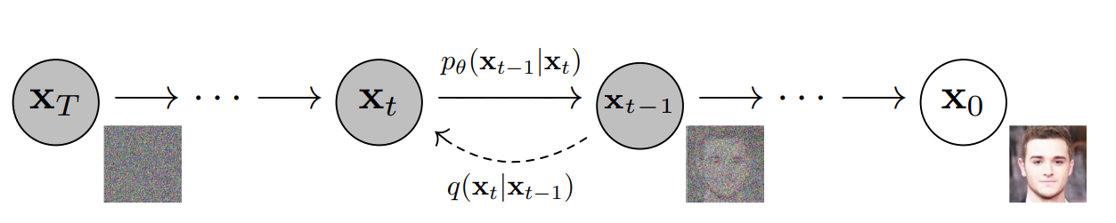
A diffusion model learns to generate data by reversing a controlled corruption process. During training, clean examples are mixed with noise at different intensities. A neural network learns what noise was added—or, in equivalent parameterizations, what clean sample or velocity produced the noisy input. During generation, the model begins with random noise and repeatedly transforms it into a structured sample.
That description is simple, but three details matter:
- Training does not run the entire noising chain for every example. Any noise level can be sampled directly.
- The reverse transition is learned because the exact reverse distribution depends on the unknown data distribution.
- Generation is iterative. Computation within one step is parallelizable, but the denoising steps themselves are sequential.
The formulation was introduced by Sohl-Dickstein et al. and made practical for high-quality image synthesis by Ho, Jain, and Abbeel. This article develops the discrete-time DDPM formulation first, then connects it to modern architectures and samplers.
1. The forward process: progressively remove signal
Let $x_0$ be a clean data sample. For images, it is typically a tensor whose values have been scaled to a fixed range. A predefined variance schedule ${\beta_t}_{t=1}^T$ controls how much Gaussian noise is added at each step.
Define $\alpha_t = 1-\beta_t$. The forward transition is
$$ q(x_t \mid x_{t-1}) = \mathcal{N}\left(x_t; \sqrt{\alpha_t}x_{t-1}, \beta_t I\right). $$Equivalently,
$$ x_t = \sqrt{\alpha_t}x_{t-1} + \sqrt{1-\alpha_t}\,\epsilon, \qquad \epsilon \sim \mathcal{N}(0,I). $$The schedule is fixed rather than learned in the original DDPM. After enough steps, the signal-to-noise ratio becomes small and $x_T$ is approximately standard Gaussian noise.

Forward noising and learned reverse denoising processes. Adapted from Ho et al..
The useful closed form
Running all $t$ forward transitions during training would be wasteful. Because the transitions are Gaussian, they compose into a closed-form distribution. With
$$ \bar{\alpha}_t = \prod_{s=1}^{t}\alpha_s, $$we can sample any noise level directly:
$$ q(x_t \mid x_0) = \mathcal{N}\left( x_t; \sqrt{\bar{\alpha}_t}x_0, (1-\bar{\alpha}_t)I \right), $$or
$$ x_t = \sqrt{\bar{\alpha}_t}x_0 + \sqrt{1-\bar{\alpha}_t}\,\epsilon. $$This equation turns training into a supervised regression problem: choose a clean sample, choose a noise level, add known noise, and ask the network to predict a target derived from those quantities.
2. What the network learns
The reverse process is represented as
$$ p_\theta(x_{t-1}\mid x_t) = \mathcal{N}\left(x_{t-1}; \mu_\theta(x_t,t), \Sigma_\theta(x_t,t) \right). $$The network can parameterize this transition in several equivalent ways. Common targets are:
- Noise prediction: estimate the sampled noise $\epsilon$.
- Data prediction: estimate the clean sample $x_0$.
- Velocity prediction: estimate a linear combination of signal and noise, often called $v$.
- Score prediction: estimate $\nabla_{x_t}\log p_t(x_t)$, the direction toward higher density at noise level $t$.
For the original noise-prediction formulation, the widely used simplified objective is
$$ \mathcal{L}_{\text{simple}} = \mathbb{E}_{x_0,t,\epsilon} \left[ \left\|\epsilon-\epsilon_\theta(x_t,t,c)\right\|_2^2 \right], $$where $c$ is optional conditioning information such as a class label, text embedding, image, mask, or another signal.
This objective is related to the variational lower bound derived for the latent-variable model and to denoising score matching. It is not correct to say that a diffusion model never sees clean data: training starts from real $x_0$ samples and constructs noisy versions of them. What the network usually receives as input is $x_t$, not an unrelated collection of noise-only examples.
One training step
The core operation is compact:
def diffusion_loss(model, x0, condition, alpha_bar):
    t = sample_timesteps(batch_size=x0.shape[0])
    noise = randn_like(x0)

    a = alpha_bar[t].reshape(-1, 1, 1, 1)
    xt = sqrt(a) * x0 + sqrt(1 - a) * noise

    predicted_noise = model(xt, t, condition)
    return mean_squared_error(predicted_noise, noise)
Real implementations also choose timestep weighting, a noise schedule, a variance parameterization, conditioning dropout, and numerical precision. The important point is that each minibatch can train on randomly selected timesteps without simulating the preceding forward steps.
3. Reverse sampling: from noise to a sample
At inference time, sampling begins with
$$ x_T \sim \mathcal{N}(0,I). $$The sampler then evaluates the neural network at decreasing noise levels. In a DDPM-style ancestral sampler, each step uses the model prediction to construct the mean of $p_\theta(x_{t-1}\mid x_t)$ and usually adds an appropriate amount of random noise. The final transition produces $x_0$.
This process is sequential: $x_{t-1}$ depends on $x_t$. Multiple samples can be batched, and every network evaluation can use GPU parallelism, but the time dimension cannot be evaluated all at once in the standard formulation.
The training timestep count and the inference-step count are not the same requirement. Early DDPM systems commonly used hundreds or thousands of neural-network evaluations. Faster approaches changed the sampling path:
- DDIM constructs a non-Markovian process with the same training objective and enables deterministic or stochastic sampling with fewer steps.
- The probability-flow ODE view connects score models to numerical differential-equation solvers (Song et al.).
- DPM-Solver exploits the structure of the diffusion ODE and reported strong results with roughly 10–20 function evaluations in its experiments.
- Distillation and consistency models target one- or few-step generation, usually with additional training and a quality or coverage trade-off.
There is therefore no universal rule that a diffusion model needs 1,000 sampling steps. Quality depends on the trained model, prediction parameterization, scheduler, solver, guidance scale, and evaluation target.
4. Architecture: U-Nets, transformers, and latent space
The diffusion equations do not require a specific neural architecture. They require a time-conditioned function capable of processing noisy data.
U-Net denoisers
Image diffusion models have traditionally used variants of the U-Net. The downsampling path builds broad spatial context; the upsampling path recovers resolution; skip connections preserve fine-grained information. A timestep embedding tells the network which noise level it is processing. Residual blocks and attention layers are commonly added at selected resolutions.
The U-Net does not provide “local and global attention to noise” by itself. Its multiscale feature hierarchy mixes local detail with wider context, while explicit attention blocks model longer-range interactions.
Diffusion transformers
U-Nets are not the only choice. Diffusion Transformers replace much of the convolutional denoiser with a transformer operating on latent patches. The diffusion process and training target can remain largely unchanged while the backbone changes.
Pixel-space and latent diffusion
A pixel-space model runs the diffusion process directly on image tensors. This is conceptually clean but expensive at high resolution.
Latent diffusion first encodes an image into a lower-dimensional representation $z_0$, trains the diffusion model in that space, and decodes the generated latent back to pixels:
$$ x_0 \xrightarrow{E} z_0 \xrightarrow{\text{diffusion}} \hat{z}_0 \xrightarrow{D} \hat{x}_0. $$Reducing spatial dimensions lowers the cost of every denoising evaluation. The trade-off is that the autoencoder becomes part of the quality ceiling: details lost during encoding cannot be perfectly recovered by the diffusion model.
5. Conditioning and guidance
A conditional diffusion model learns $p_\theta(x\mid c)$, where $c$ may represent text, a class, an image, a depth map, or another modality. The condition can enter through feature modulation, concatenation, or cross-attention. Latent diffusion models showed how cross-attention can support flexible text and spatial conditioning.
Classifier-free guidance trains the same network on conditional and deliberately dropped conditions. At sampling time, conditional and unconditional predictions are combined:
$$ \epsilon_{\text{guided}} = \epsilon_\theta(x_t,t,\varnothing) + w\left[ \epsilon_\theta(x_t,t,c) - \epsilon_\theta(x_t,t,\varnothing) \right]. $$Increasing $w$ often improves adherence or apparent fidelity, but it can reduce diversity and introduce oversaturation or other artifacts. Guidance is a controllable trade-off, not free quality. The method was formalized by Ho and Salimans.
6. How diffusion models compare with other generators
“Diffusion models outperform GANs” is too broad. A model class can lead on one benchmark and lose on latency, memory, data efficiency, likelihood, or a different domain.
| Model family | Training signal | Generation pattern | Typical strength | Typical limitation |
|---|---|---|---|---|
| Diffusion | Denoising or score regression | Iterative refinement across noise levels | Stable objective and flexible conditioning | Repeated network evaluations |
| GAN | Adversarial discriminator signal | Usually one generator pass | Fast inference and sharp samples | Minimax training can be unstable; coverage can suffer |
| Autoregressive | Next-element likelihood | Sequential over tokens or positions | Direct likelihood training and strong discrete generation | Latency grows with generated sequence length |
Dhariwal and Nichol demonstrated that carefully designed, guided diffusion models surpassed contemporary GAN baselines on several ImageNet metrics. That is an important empirical result, not a universal ordering of model families.
7. Evaluation and failure analysis
Sample quality should not be reduced to a single attractive output. For image generation, a serious evaluation may include:
- Distributional quality: FID or related feature-space measures, reported with dataset and sample-count details.
- Coverage: precision and recall-style metrics to separate fidelity from diversity.
- Condition adherence: whether generated content matches the class, text, layout, or control signal.
- Human evaluation: blinded preference or task-specific judgement with a documented protocol.
- Efficiency: neural-function evaluations, latency, peak memory, throughput, and energy or compute budget.
- Safety and data analysis: memorization, near-neighbor checks, demographic performance slices, and failure-category review.
The sampling configuration belongs in the evaluation record. Comparing two models while hiding their solver, number of steps, guidance scale, resolution, or post-processing makes the result difficult to interpret.
8. Practical limitations
Diffusion models solve important problems, but their trade-offs are concrete:
- Sequential inference cost. Fast solvers reduce the number of evaluations, but every remaining step still calls a large network.
- Training cost. High-resolution and multimodal models require substantial data, compute, storage, and experiment discipline.
- Configuration sensitivity. Noise schedules, timestep weighting, prediction targets, solvers, and guidance interact. A good sampler cannot repair a poorly trained model.
- Conditioning is imperfect. Models can omit entities, confuse spatial relations, or satisfy text while violating physical or structural constraints.
- Guidance changes the distribution. Stronger guidance can improve prompt adherence while reducing diversity or amplifying artifacts.
- Latent bottlenecks lose information. Compression makes generation cheaper but can weaken text rendering, small details, or reconstruction fidelity.
- Data risks remain. Bias, unsafe content, memorization, licensing, and provenance are dataset and deployment problems, not issues the denoising objective removes.
9. A useful mental model
The forward process defines a family of progressively noisier distributions. Training teaches a network how signal and noise relate at each level. A sampler uses that learned field to travel from a simple prior distribution back toward the data distribution.
This separates three components that are often conflated:
- the model predicts noise, data, velocity, or score;
- the scheduler defines the noise levels and coefficients;
- the sampler or solver decides how to move between those levels.
Changing the sampler can accelerate an existing model without retraining it. Changing the backbone alters the learned predictor. Changing the data or conditioning changes what distribution the system can represent. Keeping these layers separate makes diffusion systems much easier to reason about and evaluate.
References
- Jascha Sohl-Dickstein et al., Deep Unsupervised Learning using Nonequilibrium Thermodynamics, 2015.
- Jonathan Ho, Ajay Jain, and Pieter Abbeel, Denoising Diffusion Probabilistic Models, 2020.
- Jiaming Song, Chenlin Meng, and Stefano Ermon, Denoising Diffusion Implicit Models, 2020.
- Yang Song et al., Score-Based Generative Modeling through Stochastic Differential Equations, 2021.
- Alex Nichol and Prafulla Dhariwal, Improved Denoising Diffusion Probabilistic Models, 2021.
- Prafulla Dhariwal and Alex Nichol, Diffusion Models Beat GANs on Image Synthesis, 2021.
- Robin Rombach et al., High-Resolution Image Synthesis with Latent Diffusion Models, 2022.
- Jonathan Ho and Tim Salimans, Classifier-Free Diffusion Guidance, 2022.
- Cheng Lu et al., DPM-Solver, 2022.
- William Peebles and Saining Xie, Scalable Diffusion Models with Transformers, 2022.
- Yang Song et al., Consistency Models, 2023.